Model selection with non-SBML models and unsupported calibration tools
PEtab Select is currently designed for use with models encoded in SBML. However, this requirement is inherited from PEtab, and the SBML model is irrelevant to PEtab Select, which only reads the parameter table of a model’s PEtab problem to determine the estimated parameters (e.g. to accurately compute criteria values).
Furthermore, PEtab Select is designed for use with one of the supported calibration tools. However, PEtab Select also implements a command-line interface (CLI) and Python interface such that other calibration tools can easily interface with PEtab Select in order to perform the model selection.
In this notebook, we demonstrate model selection with a modeling framework that currently does not support PEtab problems (specifically, statsmodels). Since statsmodels is a Python package, we use the Python interface of PEtab Select. Synthetic data was generated from the model
where \(\epsilon\) is drawn from the standard normal distribution and represents measurement noise. The hypothetical scenario is that you are provided \((t,y)\) data pairs and asked to identify the powers of \(t\) that are evidenced by the data (i.e., that were used to generate the data). Here, we only consider polynomial models involving terms up to \(t^5\), i.e., the superset model is
where \(k_i\) is the \(i\)th coefficient in the linear regression model.
“True” model
We start by loading the data and demonstrating model calibration of the true model using statsmodels.
[1]:
# Based on the statsmodels "Ordinary Least Squares" example
# https://www.statsmodels.org/stable/examples/notebooks/generated/ols.html

import numpy as np
import petab
import statsmodels.api as sm
from petab import MEASUREMENT, TIME

import petab_select
from petab_select.constants import (
    CANDIDATE_SPACE,
    ESTIMATE,
    TERMINATE,
    UNCALIBRATED_MODELS,
    Criterion,
)

# Data was generated with the formula (see next cell to regenerate data)
# y(t) = 20*t + 10*t^2 + 5*t^3
df = petab.get_measurement_df(
    "other_model_types_problem/petab/measurements.tsv"
)
t = df[TIME].to_numpy()
y = df[MEASUREMENT].to_numpy()

# Show statsmodels fit for the "true" model
true_T = np.column_stack([t**1, t**2, t**3])
print(sm.OLS(y, true_T).fit().summary())
                                 OLS Regression Results
=======================================================================================
Dep. Variable:                      y   R-squared (uncentered):                   1.000
Model:                            OLS   Adj. R-squared (uncentered):              1.000
Method:                 Least Squares   F-statistic:                          2.226e+08
Date:                Tue, 30 Jun 2026   Prob (F-statistic):                        0.00
Time:                        15:50:30   Log-Likelihood:                         -137.59
No. Observations:                 101   AIC:                                      281.2
Df Residuals:                      98   BIC:                                      289.0
Df Model:                           3
Covariance Type:            nonrobust
==============================================================================
                 coef    std err          t      P>|t|      [0.025      0.975]
------------------------------------------------------------------------------
x1            19.8935      0.165    120.611      0.000      19.566      20.221
x2            10.0536      0.051    197.694      0.000       9.953      10.155
x3             4.9954      0.004   1334.839      0.000       4.988       5.003
==============================================================================
Omnibus:                        1.563   Durbin-Watson:                   1.861
Prob(Omnibus):                  0.458   Jarque-Bera (JB):                1.284
Skew:                          -0.078   Prob(JB):                        0.526
Kurtosis:                       2.470   Cond. No.                         695.
==============================================================================

Notes:
[1] R² is computed without centering (uncentered) since the model does not contain a constant.
[2] Standard Errors assume that the covariance matrix of the errors is correctly specified.
[2]:
# Uncomment to regenerate data

# import numpy as np
# rng = np.random.default_rng(seed=0)

# # Measurement time points
# t = np.linspace(0, 10, 101)
# # The first three powers of x are used to generate the data
# T = np.column_stack([t**1, t**2, t**3])
# K = np.array([20, 10, 5])
# noise = rng.normal(size=t.size)
# y = np.dot(T, K) + noise

# # Write PEtab measurement table
# lines = ["observableId\tsimulationConditionId\ttime\tmeasurement"]
# for t_, y_ in zip(t, y, strict=True):
#     lines.append(f"y\tdefault\t{round(t_,1)}\t{round(y_,5)}")
# content = "\n".join(lines)
# with open("other_model_types_problem/petab/measurements.tsv", "w") as f:
#     f.write(content)
Model selection
To perform model selection, we define three methods to:
calibrate a single model
This is where we convert a PEtab Select model into a statsmodels model, fit the model with statsmodels, then save the log-likelihood value in the PEtab Select model.
perform a single iteration of a model selection method involving calibration of multiple models
This is generic code that executes the required PEtab Select commands.
perform a full model selection run, involving all iterations of a model selection method
This loads the PEtab Select problem from disk and performs all iterations of a model selection method.
In this case, the PEtab Select problem is setup to perform backward selection (see the specification files for this example).
[3]:
def calibrate_model(model: petab_select.Model, t=t, y=y):
    # Convert the PEtab Select model into a statsmodel model
    powers = [
        int(parameter_id[1:])
        for parameter_id, parameter_value in model.parameters.items()
        if parameter_value == ESTIMATE
    ]
    if not powers:
        return
    T = np.column_stack([t**i for i in powers])
    sm_model = sm.OLS(y, T)

    # Calibrate
    results = sm_model.fit()

    # Save the log-likelihood
    model.set_criterion(criterion=Criterion.LLH, value=results.llf)


def perform_iteration(
    problem: petab_select.Problem, candidate_space: petab_select.CandidateSpace
):
    # Start the iteration, request models according to the model selection method.
    iteration = petab_select.ui.start_iteration(
        problem=problem, candidate_space=candidate_space
    )

    # Calibrate each model.
    models = iteration[UNCALIBRATED_MODELS]
    for model in models:
        if all(
            parameter_value != ESTIMATE
            for parameter_value in model.parameters.values()
        ):
            del models[model.hash]
            continue
        calibrate_model(model=model)
        # Compute the criterion based on the log-likelihood computed by statsmodels.
        model.compute_criterion(criterion=problem.criterion)

    # End the iteration and return the results.
    return petab_select.ui.end_iteration(
        problem=problem,
        candidate_space=iteration[CANDIDATE_SPACE],
        calibrated_models=models,
    )


def run_model_selection():
    # Load the PEtab Select problem.
    problem = petab_select.Problem.from_yaml(
        "other_model_types_problem/petab_select/problem.yaml"
    )
    candidate_space = None

    # Perform all iterations of the model selection method until the termination signal is emitted.
    while True:
        iteration_results = perform_iteration(
            problem=problem, candidate_space=candidate_space
        )
        if iteration_results[TERMINATE]:
            break
        candidate_space = iteration_results[CANDIDATE_SPACE]

    # Return the problem, which contains the calibrated models.
    return problem
[4]:
# Run the model selection method.
problem = run_model_selection()
Analysis
As when using a PEtab-compatible calibration tool, the results from calibration with statsmodels can also be analyzed with PEtab Select.
Firstly, we get the best model identified during model selection. It matches the “true” model, with the same AIC as computed by statsmodels at the top of this notebook.
[5]:
best_model = petab_select.analyze.get_best(
    models=problem.state.models, criterion=problem.criterion
)
print(f"""
Best model information
----------------------
PEtab Select model hash: {best_model.hash}
Selected powers of t: {[int(parameter_id[1:]) for parameter_id, parameter_value in best_model.parameters.items() if parameter_value == ESTIMATE]}
Log-Likelihood: {best_model.get_criterion(criterion=Criterion.LLH)}
AIC: {best_model.get_criterion(criterion=Criterion.AIC)}
""")
Best model information
----------------------
PEtab Select model hash: M-011100
Selected powers of t: [1, 2, 3]
Log-Likelihood: -137.59037189701047
AIC: 281.18074379402094
[6]:
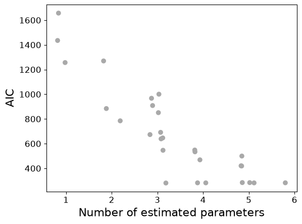
# Plot AIC of all models that were calibrated.

import petab_select.plot

plot_data = petab_select.plot.PlotData(
    models=problem.state.models, criterion=problem.criterion
)

petab_select.plot.scatter_criterion_vs_n_estimated(plot_data=plot_data);
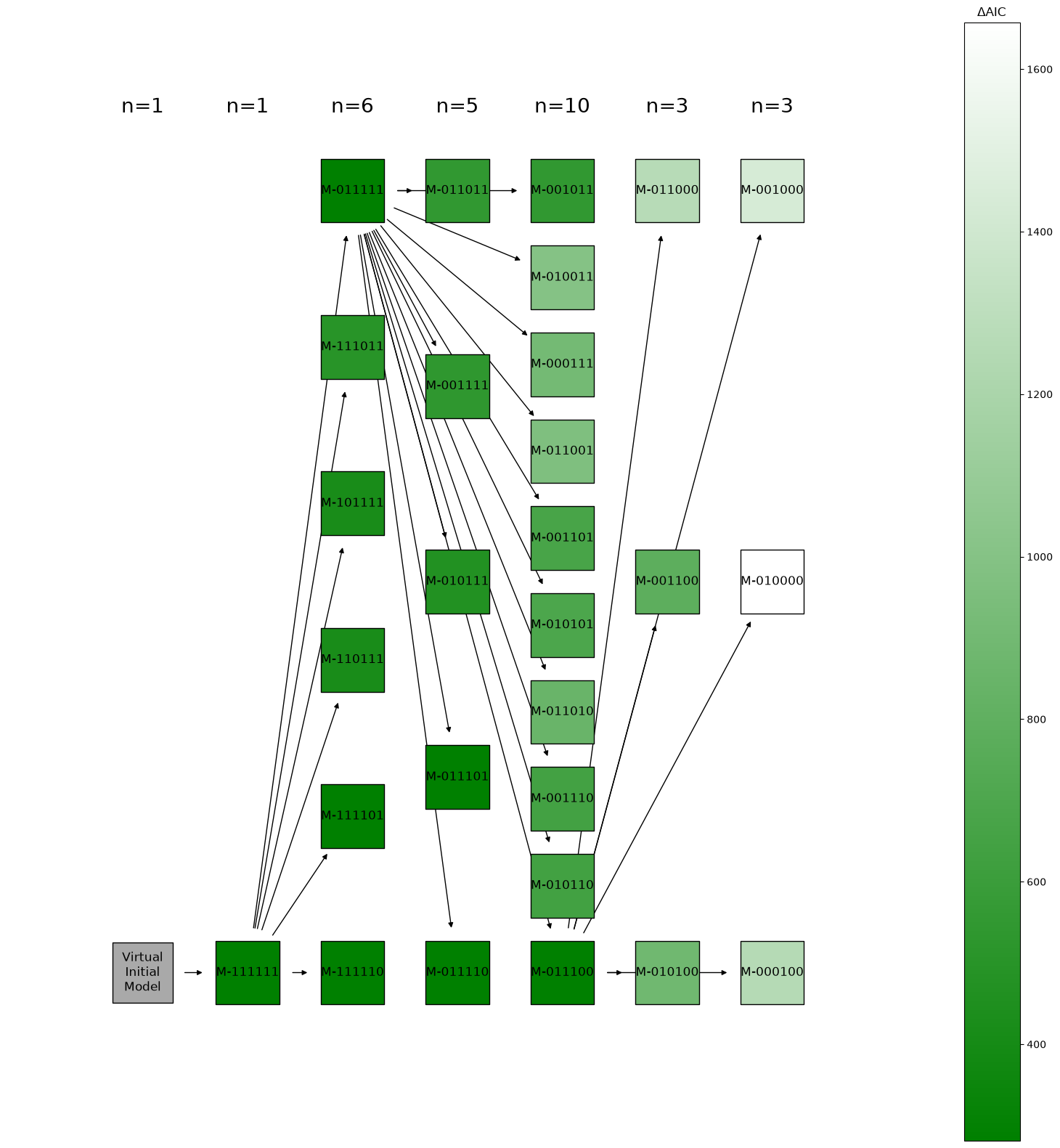
[7]:
# Plot the history of model selection iterations.
import matplotlib.pyplot as plt

draw_networkx_kwargs = {
    "arrowstyle": "-|>",
    "node_shape": "s",
    "edgecolors": "k",
}
fig, ax = plt.subplots(figsize=(20, 20))
petab_select.plot.graph_iteration_layers(
    plot_data=plot_data,
    draw_networkx_kwargs=draw_networkx_kwargs,
    ax=ax,
);
Supplementary: the PEtab files
The PEtab Select problem used above is stored alongside this notebook, in other_model_types_problem/. This section explains what those files contain. The directory has two parts: a standard PEtab problem (petab/) that describes the model and data, and a PEtab Select problem (petab_select/) that describes the model space and the selection settings.
other_model_types_problem/
├── petab/                 # the PEtab problem
│   ├── problem.yaml
│   ├── parameters.tsv
│   ├── observables.tsv
│   ├── conditions.tsv
│   ├── measurements.tsv
│   └── dummy.xml
└── petab_select/          # the PEtab Select problem
    ├── problem.yaml
    └── model_space.tsv
The PEtab problem (petab/)
A PEtab problem normally pairs an SBML model with tables for parameters, observables, conditions, and measurements. In this example however, we focus on only the information relevant to PEtab Select. The required non-dummy files are:
problem.yaml— the PEtab problem file. It points to the parameter table and, for its single problem, to the condition, measurement, (dummy) observable, and (dummy) SBML files.parameters.tsv— the six regression coefficientsk0–k5, one per power oft. Each is on a linear scale with bounds[0, 100]. Theestimatecolumn is only a default; for each candidate model, PEtab Select overrides it (via the model space) to decide which coefficients are estimated. This is the only table PEtab Select reads, in order to count the estimated parameters when computing criteria such as the AIC.
The other files can be dummy files. In this example, we used them to encode as much information as possible, even though they are not used, just to demonstrate the PEtab format:
observables.tsv— defines a single observableywhose formula is the regression model \(y(t) = \sum_{i=0}^{5} k_i\, t^i\), written ask0*time^0 + k1*time^1 + ... + k5*time^5. ThenoiseFormulais1(unit, constant noise), matching the standard-normal noise used to generate the data.conditions.tsv— a single dummy experimental condition,default(the data involves no experimental perturbations/conditions).measurements.tsv— the synthetic data: 101 measurements of observableyat conditiondefault, one per time point \(t = 0.0, 0.1, \ldots, 10.0\). The values were generated from \(y(t) = 20t + 10t^2 + 5t^3 + \epsilon\) (i.e. only the powers \(t^1, t^2, t^3\) are truly present) with standard-normal noise \(\epsilon\). This is used in the notebook to load data, but the data could have been loaded from e.g. an Excel spreadsheet too.dummy.xml— an essentially empty SBML model.
We display each PEtab table below, and print the PEtab problem YAML file.
[1]:
import pandas as pd
from IPython.display import display

for petab_file in [
    "petab/parameters.tsv",
    "petab/observables.tsv",
    "petab/conditions.tsv",
    "petab/measurements.tsv",
]:
    print(petab_file)
    display(pd.read_csv(f"other_model_types_problem/{petab_file}", sep="\t"))
petab/parameters.tsv
| parameterId | parameterScale | lowerBound | upperBound | estimate | |
|---|---|---|---|---|---|
| 0 | k0 | lin | 0 | 100 | 1 |
| 1 | k1 | lin | 0 | 100 | 1 |
| 2 | k2 | lin | 0 | 100 | 1 |
| 3 | k3 | lin | 0 | 100 | 1 |
| 4 | k4 | lin | 0 | 100 | 1 |
| 5 | k5 | lin | 0 | 100 | 1 |
petab/observables.tsv
| observableId | observableFormula | noiseFormula | |
|---|---|---|---|
| 0 | y | k0*time^0 + k1*time^1 + k2*time^2 + k3*time^3 ... | 1 |
petab/conditions.tsv
| conditionId | |
|---|---|
| 0 | default |
petab/measurements.tsv
| observableId | simulationConditionId | time | measurement | |
|---|---|---|---|---|
| 0 | y | default | 0.0 | 0.12573 |
| 1 | y | default | 0.1 | 1.97290 |
| 2 | y | default | 0.2 | 5.08042 |
| 3 | y | default | 0.3 | 7.13990 |
| 4 | y | default | 0.4 | 9.38433 |
| ... | ... | ... | ... | ... |
| 96 | y | default | 9.6 | 5537.44101 |
| 97 | y | default | 9.7 | 5697.67947 |
| 98 | y | default | 9.8 | 5861.01878 |
| 99 | y | default | 9.9 | 6028.19348 |
| 100 | y | default | 10.0 | 6200.50268 |
101 rows × 4 columns
[9]:
# The PEtab problem YAML file
print(open("other_model_types_problem/petab/problem.yaml").read())
format_version: 1
parameter_file: parameters.tsv
problems:
- condition_files:
  - conditions.tsv
  measurement_files:
  - measurements.tsv
  sbml_files:
  - dummy.xml
  observable_files:
  - observables.tsv
The PEtab Select problem (petab_select/)
model_space.tsv— the model space. It defines a single model subspaceM(pointing to../petab/problem.yaml) with one column per coefficient,k0–k5. Each entry is0;estimate, meaning the coefficient can either be fixed to0(that power oftis then effectively removed from the model) or estimated (that power is present). With six independently toggled coefficients, this single row compactly encodes all \(2^6 = 64\) candidate models. The goal of the selection is to recover the powers that generated the data (\(t^1, t^2, t^3\)).
[10]:
print("petab_select/model_space.tsv")
display(
    pd.read_csv(
        "other_model_types_problem/petab_select/model_space.tsv", sep="\t"
    )
)
petab_select/model_space.tsv
| model_subspace_id | petab_yaml | k0 | k1 | k2 | k3 | k4 | k5 | |
|---|---|---|---|---|---|---|---|---|
| 0 | M | ../petab/problem.yaml | 0;estimate | 0;estimate | 0;estimate | 0;estimate | 0;estimate | 0;estimate |
problem.yaml— the model selection settings: compare models by theAICcriterion, search the model space with thebackwardmethod(start from the full model and remove terms), and read the model space frommodel_space.tsv.
[11]:
# The PEtab Select problem YAML file
print(open("other_model_types_problem/petab_select/problem.yaml").read())
format_version: 1
criterion: AIC
method: backward
model_space_files:
- model_space.tsv